Research on Electromagnetic Driving Robot Fish-Juniper Publishers
Juniper Publishers-Journal of Robotics

Abstract
Based on the actual physical appearance of the tuna
and the wave equation derived from observing its swimming locomotion,
this paper proposes a new idea on the simulation and modeling of the
robot fish and a novel way of thinking on kinetic analysis. The motion
law for each joint of the robot fish was first obtained through the
discrete fitting method and the motion law was subsequently used as the
basis for the robot fish electromagnetic drive control signal. The
fluent flow field analysis software was utilized. The meshing of the
fluid around the fish body was performed by using the dynamic grid
technique. The surface pressure values of the fish body during the
steady state forward movement were analyzed, and the values of the
driving force of each part of the fish were obtained. It was then
determined that the electromagnetic drive caudal fin robot fish was the
optimal design. Based on the idea of digital-analog conversion, the
drive control signal waveform was digitally discretized, then the C51
single-chip microcomputer and DAC digital-to-analog converter was used
for conversion. The OPA544 op amp chip was then used to simulate the
amplified output in accordance with the control signal waveform.
Electromagnetic coil drive signal with variable frequency and voltage
can thus be achieved.
Keywords: Robot fish; Electromagnetic drive; Fluent flow field analysis; Kinetic analysis; Control signal; Swimming experiment
Construction of the Robot Fish Model
Determination ofthe external physical characteristics of the fish body and the number of joints
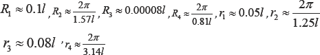
A real tuna fish was selected, the total length was
measured and the external curve of the fish body was fitted; the
following data can be obtained:
Total length l = 260mm
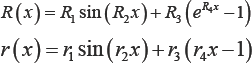
Where R(x) is the function of the longitudinal fish body curve, r(x) is the function of the transverse fish body curve
In the selection of the number of joints of the robot
fish, the higher the number of joints, the higher the degree of fit
between the swimming curve and the known fish body wave equation, the
closer it is to the real fish-swimming situation. On the other hand, the
cumulative error of the series structure and the complexity of the
structure should also be considered. Usually the range for the number of
robot joints N is 2-10. The number of robot fish joints designed in
this paper is N = 6.
In the design of the length of each joint,
considering that the movement of the fish body is mainly concentrated in
the rear half of the fish body, therefore the first half 130 mm of the
fish can be viewed as not swinging. Also, according to the actual
measurement, it is known that the fish tail length is 47 mm. Based on
the joint size parameter optimization design method proposed by Chai
Zhikun [1],
except for the tail joint, the proportion of the remaining five joints
should be 83: 67: 59: 53: 48. The length of each joint after calculation
and rounding is: joint 1 is 22mm, joint 2 is 18mm, joint 3 is 16mm,
joint 4 is 14mm, joint 5 is 13mm, and the joint 6 (caudal fin) is 47mm
long.
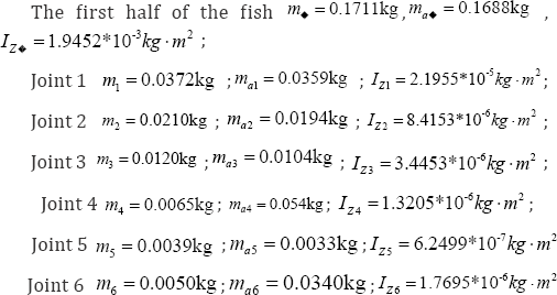
Calculation of the mass and moment of inertia of each part
Based on the above geometric parameters of the fish, the mass of the various parts of the fish can be calculated:
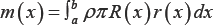
Where, ρ is the fish density (kg/m3),
which can be approximated as the density of water, a, b are the
abscissa values of the starting point and the end of each joint.
During the swimming process of the fish, due to
interaction with the surrounding fluid, the fish has a virtual mass.
According to Lighthill's "Large-amplitude elongated-body theory of fish
locomotion,” the equation for calculation of the virtual mass of the
fish body cross-section is [2]:
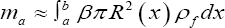
Where ρf is the fluid density, β is the virtual mass coefficient; when there is no fish fins on the fish cross-section,
β = 1.
As the robot fish cross-section can be regarded as an
oval with the long axis of 2R (x), the short axis of 2r (x), the
inertia of each part around the z-axis can be calculated according to
the following formula:
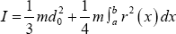
Where m is the sum of the mass of each joint and the
virtual mass, and do is the length of each joint. As this robot fish has
six joints, therefore there is seven parts in total. The following is
the calculated mass of each joint, virtual mass, and moment of inertia:
Kinematical Analysis of the Robot Fish
According to the observations of the tuna fish by Donley and Sepulveda and others [3], the fish body wave equation corresponding to the swimming locomotion of this type of fish is: h (x, t )= H (x) sin (ωt - kx) , where, h (x, t) is the lateral displacement of the fish. H (x) is the envelope equation of the fish’s swimming locomotion. ω is the swing frequency of each fish joint, k is the wave number of the fish body. k = 5.7/1 . H (x) = α1 + α2 + α3x2 , Where α1 = 0.02/ α2 =-0.12 α3 = 0.3/1.
When the frequency of each joint is 2Hz, the swing
period is 0.5s. The swing cycle is divided into 10 moments. With the
starting point of each joint as the center, the joint length is the
intersection of the radius and the fish wave equation at that moment.
The coordinate position of the six joint starting points at each moment
was obtained (In this coordinate system, the front end of the fish head
is the coordinate origin, the forward direction of the swimming
direction is the negative direction of the x axis, and the direction of
the lateral displacement is the y direction, dynamic body coordinate
system). The following Table 1 is the calculated coordinates of each joint starting point at each moment.


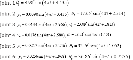
The swing movement law of each joint can be obtained by using curve fitting toolbox cftool of Matlab, As shown in Figure 1.
Fluent Flow Field Simulation and Kinetic Analysis of Robot Fish
The Cartesian coordinate system was established: the
negative direction of the x-axis was the advancing direction of the
fish, the z-axis was the transverse displacement direction of the fish,
and the y-axis was the longitudinal displacement direction of the fish.
Ignoring the force in the y-axis direction of the fish (gravity,
buoyancy, lift due to pectoral fins, and others), and considering only
the x-z plane force on the body during the advancing process, the fish
is only subjected to two forces: the resulting thrust due to swing water
and the resistance in the forward movement.
According to the "large-amplitude elongated-body
theory of fish locomotion,” the fish's thrust is the component of the
hydrodynamic force generated by the fish's swing in the forward
direction [4].
However, due to the complexity of the flow field, there is no standard
and uniform thrust formula. It is difficult to obtain relatively
accurate simulation results. Therefore, the fluent flow field analysis
method was used. The dynamic grid technology was used for the meshing of
the fluid around a certain area of the fish, and turbulence model was
used to obtain the solution. Hence, the forces exerted by the
surrounding fluid on the fish body during the steady state forward
movement can be obtained by simulation (surface pressure and viscous
force). Further, the thrust formula can be obtained.

As shown in Figure 2a is a three-dimensional model of the extracted robot fish, Figure 2b
is a plane view intercepted at y = 0 after the static grid division is
completed. In the choice of computing domain, on the one hand, the
length of the calculation area must be large enough to meet the needs of
the continuous advance of the robot fish; on the other hand, the
smaller calculation area can improve the calculation efficiency. After
several trials, the calculation domain was selected as rectangular, the
length, width, and height were selected to be 10 times of the
corresponding maximum size of the biomimetic robot fish.

In the above model, the triangular/tetrahedral mesh
is used to divide the area/body domain of the region. Since the grid
boundary changes with time according to the variation trend of the fish
wave equation, it is necessary to define the grid as the dynamic grid in
the computing domain. Also, the spring smooth method and the local mesh
reconstruction method were used to ensure the quality of dynamic grid.
The following is the dynamic grid parameters: the spring coefficient is
0.2, the boundary node relaxation factor is 0.4, the maximum length of
the local reconstruction is 0.021, the minimum length is 0.0004, the
maximum cell skew rate is 0.76, and the size function is activated, and
the remaining values are default.
On the boundary condition, the boundary conditions of
the six surfaces of the rectangular parallelepiped and the surfaces of
the biomimetic robot fish are all non-slip condition on the wall
surface, but the dynamic region is defined by the UDF (User Defined
Functions) function. For the robot fish model, DEFINE-GRID-MOTION Macro
was used to define the movement of fish. Take the movement at the end of
the joint as an example; the custom program of this dynamic region can
be defined as follows:
#include "udf.h”
#define PI 3.1415926
DEFINE_GRID_MOTION (guanjie6,domain,dt,time,dtime)
{
Thread *tf = DT_THREAD(dt);
face_t f;
Node *v;
real NV_VEC(omega), NV_VEC(axis), NV_VEC(dx);
real NV_VEC(origin), NVVEC(rvec);
int n;
SET_DEFORMING_THREAD_FLAG(THREAD_T0(tf));
begin_f_loop(f,tf)
{
f_node_loop(f,tf,n)
{
v = F_NODE(f,tf,n);
if (NODE_POS_NEED_UPDATE (v))
{
NODE_POS_UPDATED(v);
NV_S(omega, =, 0.0);
NV_D(axis, =, 0.0, 1.0, 0.0);
origin[0] = 0.213;
origin[1] = NODE_Y(v);
origin[2] = 0;
omega[1] = 0.2587*PI*PI*sin(4*PI*time-0.3848+PI/2);
NV_VV(rvec, =, NODE_COORD(v), -, origin);
NV_CROSS(dx, omega, rvec);
NV_S(dx, *=, dtime);
NV_V(NODE_COORD(v), +=, dx);
}
}
}
end_f_loop(f,t)
}
In the choice of the calculation model, because the
robot fish movement belongs to the large Reynolds number movement mode,
therefore the transient three-dimensional turbulence model was used for
solution. Due to the wide range of applications (especially the
situation of high Reynolds number), economic, reasonable accuracy, and
other characteristics, k-epsilon turbulence model was used.
Since the surface of the fish is divided into seven
parts according to the joint position when drawing the three-dimensional
map, the force component of the wall area of the fish body in the
specified direction (the advancing direction of the robot fish) can be
obtained in the processing of the results.
In Table 2, x(p) represents the fish surface pressure value, and x (v) represents the viscous force value. It can be seen from Figure 3 and Table 2
that the positive and negative surface pressure of the fish in the
z-direction is cancelled in one cycle, and the viscous force is usually
in the resistance state, and its value is small relative to the surface
pressure, the difference is 2-3 orders of magnitude. Consequently, it
can be neglected when fitting the thrust formula. The thrust value of
each part of the fish body can be obtained as follows (N):
Fish front end: T0 = 0.1094sin(4nt + 5.098)-0.0410 ;
Joint 1: T1 = 0.0875sin (8πt - 0.3221)-0.0477 ;
Joint 2: T2 = 0.1639sin(4πt + 0.9005)-0.0835 ;
Joint 3: T3 = 0.2328sin(4πt + 0.2085)-0.1045 ;
Joint 4: T4 = 0.2410sin(4πt-0.3612)-0.1170 ;
Joint 5: T5 = 0.2247sin(4πt + 5.575)-0.1360 ;
Joint 6: T6 = 1.638sin (8πt +1.881)-1.571 .
The influence of viscous resistance (frictional
resistance) is small and negligible in the case of fish swimming
locomotion that has a large Reynolds number (As demonstrated in Table 2). The pressure resistance, which played a major role, can be calculated by the standard Newton equation [5]:


Dp = 0.5CpSpU 2ρ
WhereCp is the resistance coefficient, usually 1.2; Sp is
the effective area, in the practical application ( is the displacement)
can be used as the effective area of action as the fish moves in the
water, because the density of fish and water are basically the same, Sp =(m/ρ)2/3 [6].U is the average speed of swimming locomotion; ρ is the density of water.
It can be concluded that the rear joint (caudal fin)
provides the maximum thrust, accounting for more than 80% of the total
thrust, so the caudal fin drive mode is selected; electromagnetic drive
has advantages of compact structure, pollution-free, high reliability,
and large driving force, and accurate process control can be achieved.
The cyclic oscillation-driving mode is selected to be the
electromagnetic drive.
Research on Control Signal of Electromagnetic Drive Robot Fish
Signal transformation
The standard electromagnetic coil current waveform
was digitized, and then through the MCU processing the signal was
transferred to the DAC module for digital-analog transformation to
reproduce the analog control signal. The realization of the control
signal was the acquisition, storage, and reproduction of the standard
control waveform, which was used to drive the electromagnetic coil that
further drove the caudal fin movement. The basic flow of the control
drive circuit is shown in Figure 4. The components used in the Multisim simulation are described in Table 3.

Simulation circuit has been completed. A waveform
generator and an oscilloscope were used as waveform generation and
acquisition circuit (sinusoidal wave as an example) in Multisim. The
amplitude was set to 255V, the cycle was 1s, as shown in Figure 4 & 5.
After the standard sine wave was obtained, the collection and digital discretization was required. As shown in Figure 6,
the oscilloscope in Multisim provided the function of waveform
sampling. Click "Save” on the oscilloscope in the figure, the settings
of the sampling time interval and number of sampling points of the
oscilloscope will be displayed. To ensure signal accuracy, 120 points
were sampled in a cycle. The sampled data was set as a binary output
text file.
After the sampling data was obtained, start the
singlechip microcomputer-programming interface of the completed
circuit simulation platform. The collected discrete value's output was
through the single-chip microcomputer one by one cyclically. The
programming interface and the program are shown in Figure 7.


After programming, the program is successfully
downloaded to the single-chip microcomputer, click on the "start
simulation,” back to Figure 5 interface and open the two oscilloscopes in the figure, waveform as shown in Figure 8 can be observed (Figure 9).


Oscilloscope XSC2 displays the 8-bit DAC direct
output of the control signal; the oscilloscope XSC1 displays the output
control signal of the DAC output after passing through the polarity
converter. For the frequency of the waveform, delay value in the
parentheses of the delay statement in the program can be adjusted. When
calling the delay program, the singlechip microcomputer will adjust the
output hold time of each digit according to the delay value in
parentheses, and thus the frequency of the whole waveform can be
adjusted. The amplitude needs to be matched based on the characteristics
of the power amplifier module in the actual circuit and the DAC module
in the actual circuit has a reference voltage setting [7-10].
The simulation program as shown in Figure 3 & 4
was then transplanted to the Keil single-chip microcomputer programming
software. After the program was successfully compiled, the crystal
resonator frequency was set to be the crystal resonating frequency of
the single-chip microcomputer, which was 12Mhz. The Keil debugging
interface was started, break points out of the cycles were set, and the
delay parameter in the brackets of the "delay ()” statement was adjusted
continuously until the output cycle reached 1s, namely, control signal
so that the caudal fin swing cycle was 1Hz. The debugging interface of
Keil as shown in Figure 4 & 5
was entered. In every click of "run”, the program executed a cycle, and
"sec” increased accordingly, and the added value was the time required
to output a complete waveform [11-14].
After debugging, the program was downloaded to the
single-chip microcomputer. The DAC output control waveform can be
observed by connecting the DAC module output with the oscilloscope. It
can be seen that the actual circuit output control signal and the
simulation circuit output signal were exactly the same.
Signal adjustment
The DAC module was connected with the STC89C52
development board with the downloaded test program. The output of the
DAC module was connected to the input of the power amplifier module. The
DAC module and the power amplifier module shared the DC ± 15V power
supply. The overall circuit of the control platform is shown in Figure 10.
The "delay ()” delay parameter was modified in the Keil programming
debugging interface, the signal frequency was the electromagnetic coil
operating frequency.

Experimental Study
Development of experimental prototype of robot fish
The external fish body shape curve was imported into
the Pro/E three-dimensional modelling software; closed fish surface
shape can be obtained by the use of "variable crosssection scanning”
tool. Then, "thickening” operation was performed on the surface, with
the set thickness of 1.8 mm. The closed fish body shell was thus
obtained. Considering the fish body assembly, weight allocation, fish
body was designed into a removable form, as shown in Figure 11.

After modeling, the fish body model was obtained with
the use of precision 3D printing, the printing material was resin. The
polypropylene caudal fins were tailored to thin caudal fins according to
the caudal fins of the actual tuna fish, and the flexible caudal fins
were then fixed on the connecting parts as shown in Figure 12. Underwater experiments are shown in
Figure 13.


Electromagnetic drive robot fish underwater experiment
Fish body linear curve swimming experiment: In
the
experiment, the swing frequency of the fish when swimming along straight
lines is set within 1-8Hz. The amplitude of the drive voltage is set
between 2-6V. After adjustment of the fish weight, the control signal
waveform acquisition was used to generate 1-8Hz sinusoidal signal, the
signal waveform are shown in Figure 14.
By adjusting the frequency of the control signal through adjusting the
delay time of the sinusoidal output program, the obtained experimental
data is recorded in Table 4, the distribution diagram of velocity - frequency under different voltage amplitude is shown in Figure 15.
The above data is shown in Figure 15.
The greater the amplitude of the driving voltage signal, the faster the
fish swims. At different drive voltage amplitude, the best swing
frequency was basically the same; at about 2Hz, the fastest swimming
speed was achieved. As the high drive voltage heats up the coil, it is
desirable to operate at low voltage, hence at 2 V voltage, 2Hz, the
swimming speed of 81.74mm/s was selected as the best electromagnetic
drive control signal [15-18].


Conclusion
Based on the actual physical appearance of the tuna
and the wave equation derived from observing its swimming locomotion,
the motion law of each joint of the robot fish is obtained through the
discrete fitting method, and the motion law is utilized as the basis of
the control signal of the electromagnetically driven robot fish. With
the utilization of the fluent flow field analysis software, a dynamic
grid technique was used to mesh the fluid around the fish body. By
analyzing the surface pressure value of the simulated fish body in the
steady state of forward movement, the thrust values of each part of the
fish body were obtained. Hence, the electromagnetic-driven caudal fin
robot fish was determined as the optimal design. Based on the idea of
digital-analog conversion, the drive control signal waveform was first
digitally discretized. Then, it was converted through the C51
single-chip microcomputer and DAC digital-to-analog converter. Finally,
the simulated amplified analog output was obtained through the OPA544 op
amp chip in accordance with the waveform of the control signal.
Electromagnetic coil drive signal with variable frequency and voltage
was thus achieved. An electromagnetic driven caudal fin robot fish
prototype was successfully produced, a number of robot fish underwater
experiments were designed, and a series of experimental data was
obtained. Based on the linear swimming experiment of the robot fish
prototype, it was obtained that the optimal value of the electromagnetic
drive signal is 2V, 2HZ when the electromagnetic driven caudal fin
robot fish was at a relatively high speed. Based on this, the next steps
of the study lays on the following two aspects:
For more open access journals please visit: Juniper publishers
For more articles please click on: Robotics & Automation Engineering Journal


Comments
Post a Comment