Adaptive Control for Quadrotor UAVs Considering Time Delay: Study with Flight Payload- Juniper Publishers
Juniper Publishers- Journal of Robotics

Abstract
Design of effective control for unmanned aerial
vehicles (UAVs) requires consideration of several sources of
uncertainty. These undesired uncertainties affect the flight stability
and performance in an unpredictable manner. The existence of
transmission delays caused by wireless communication and payload
variation are among such critical challenges. Adaptive control (AC) can
lead to high performance tracking in the presence of uncertainties. This
paper presents the application of model reference adaptive control
(MRAC) to quadrotor types of UAVs considering the time delay in the
altitude control system. MATLAB system identification tool is applied to
obtain the altitude motion model, without time delay, for the
quadrotor. Proportional-plus-velocity (PV) and PV-MRAC altitude control
systems are designed, by incorporating an estimated constant time delay.
The designed controllers are validated using simulations and flight
tested in an indoor environment. The robustness of the PV-MRAC
controller is tested against the baseline non-adaptive PV controller
using the quadrotor’s payload capability..
Keywords: Adaptive control; Flight payload; Flight stability; MIT rule; PV control; Quadrotor; Time delayAbbreviations : UAV: Unmanned Aerial Vehicles; AC: Adaptive Control; MRAC: Model Reference Adaptive Control; PV: Proportional-Plus-Velocity; UDP: User Datagram Protocols; CTA: Continuous Time Approximation; DDE: Delay Differential Equations; LTI : Linear Time-Invariant
Introduction
The application of autonomous control techniques to
quadrotor types of unmanned aerial vehicles (UAVs) has been the focus of
active research during the past decades. Design of control for aircraft
requires several important considerations. There are numerous sources
of uncertainty. For example, devices are ageing and wearing (e.g.,
actuator degradation), external disturbances, control input saturation,
payload fluctuations, and potentially uncertain time delays in
processing or communication [1].
These undesired nonlinearities affect the flight stability and
performance of the controlled systems. Adaptive control (AC) is a
candidate to resolve the issues, because of its ability to generate high
performance tracking in the presence of uncertainties [1].
Safe, cooperative transportation of possibly large or
bulky payloads by UAVs is extremely important in various missions, such
as military operations, search and rescue, and personal assistants.
Another huge area of application is in the service industry, where
commercial quadrotor types of UAVs or drones are being used in the
delivery of packages of varying masses. There are several substantial
challenges and open research questions related to this application. For
example, this task requires that hovering vehicles remain stable and
balanced in flight as payload mass is added to the vehicle. If payload
is not loaded centered or the vehicle properly trimmed for offset loads,
the drone experiences bias forces that must be rejected [2].
Flying with a suspended load, known as slung load or sling load, can be
a very challenging and sometimes hazardous task because the suspended
load significantly alters the flight characteristics of the quadrotor [3,4].
Time delays exist in autonomous dynamic systems when
signals are transmitted wirelessly. One of the challenges in designing
effective control systems for UAVs is existence of signal transmission
delay. The delay has nonlinear effects on the flight performance of
autonomously controlled UAVs. For autonomous aerial robots, typical
values of the time delay have been known to be around 0.4±0.2s [5] or 0.2s [6].
For large delays (e.g., larger than 0.2 s) the system response might
not be stabilized or converged due to the dramatic increase in torque.
This poses a significant challenge [7]. Since its effect is not trivial the delay need be estimated and considered in designing controllers.
Parrot AR. Drone 2.0, a commercialized drone, is
controlled via WiFi network. Data streaming, commanding and reading the
vehicle sensors are done using user datagram protocols (UDPs). The drone
dynamics contains a time delay due to such communication. Refer to
Section 2 for the drone's altitude control architecture. The overall
time delay is attributed to:
I. The processing capability of the host computer,
II. The electronic devices processing the motion signals,
III. The measurement reading devices, e.g., the distance between the ultrasonic altitude sensor and the ground, and
IV. The software on the host computer for implementing the controllers.
For UAVs, wireless communication delays may not be
critical when the controllers are on board. However, delays have
significant effects when the control software is run on an external
computer and signals are transmitted wirelessly. For example, the
experiments presented in this paper were conducted using MATLAB/Simulink
on an external computer, and decoding process of the navigation data
(yaw, pitch, roll, altitude, etc.) contributes to the delay. Also, the
numerical solvers introduce additional delay. Estimating delays is a
challenging problem and has been an area of great research interest in
fields as diverse as radar, sonar, seismology, geophysics, ultrasonic,
controls, and communications [8,9]. A considerable number of system identification methods have been reported in the literature [10,11].
However, most of the existing methods for transfer function
identification do not consider the process delay (or dead-time) or just
assume knowledge of the delay [12].
Even though considerable efforts have been made on parameter
estimation, there are still many open problems and there is no common
approach in time-delay identification due to difficulty in formulation [13]. Several approaches for estimation of delay have been introduced in the literature [14-18]. In [14]
for example, the finite dimensional Chebyshev spectral continuous time
approximation (CTA) was used to solve delay differential equations
(DDEs) for estimation of constant and time-varying delays.
In this paper, the constant delay applied in the
drone's altitude control system was estimated using an approach based on
analytical solutions to DDEs [19,20]. The time delay has been estimated as 0.36s in [21,22].
The altitude dynamics was assumed to be linear time-invariant (LTI)
first order and the time delay, assumed to be single constant, was
incorporated into the model as an explicit parameter. Experimental data
and analytical solutions of infinite dimensional continuous DDEs were
used for estimation. Measured transient responses were compared to time
domain descriptions obtained by using the dominant characteristic roots
based on the Lambert W function written in terms of system parameters
including the delay. Proportional (P) time-delay control system,
retarded type, was used to generate the responses for estimation of the
delay.
The contribution of this paper is the identification
of altitude motion model, without time delay, for the drone and the
extension of incorporating the estimated time delay of 0.36 sin the
design of an AC system. Then, validating the controller using the
payload capability of the quadrotor. A model reference adaptive control
(MRAC) based on the MIT rule is designed. In general, the MIT rule
cannot guarantee stability [23],
so the MRAC is combined with a tuned proportional-plus- velocity (PV)
controller. To validate the robustness of the PV- MRAC controller, the
results are compared to a baseline nonadaptive PV-controller.
This paper continues with the description of
quadrotor's altitude dynamics and the AR. Drone 2.0 control system in
Section 2. The altitude model identification and the design of the PV
and PV-MRAC control systems are presented in Section 3. Simulations and
experiments setups are presented in Section 4. In Section 5results are
summarized. Concluding remarks and future work are presented in Section
6.
Quadrotor Altitude Dynamics and Control System
The notation for a typical quadrotor model is shown in Figure 1.
Quadrotors has three main coordinate systems attached to it; the
body-fixed frame,{b},the vehicle frame, {v} and the global inertial
frame,{ w }. There are two other coordinate systems, not shown, that are
of interest, the vehicle-1 frame,{v1} ,and vehicle-2 frame, {v2} [24,25]. The configuration of a quadrotor is represented by six degrees of freedom in terms of position, (xw ,yw,zw)T and the attitude defined using the Euler angles (roll, pitch, and yaw), (Øv2,θv1,φv)T, which gives a 12-state equation of motion [26]. The AR. Drone quadrotor platform adopted for this work has the same architecture design shown in Figure 1.

The
quadrotor has four rotors, labelled 1 to 4, mounted at the end of each
cross arm. The rotors are driven by electric motors powered by
electronic speed controllers. Each rotor is controlled independently by
nested feedback loops as shown in Figure 2.
The inner attitude control loop uses on-board accelerometers and gyros
to control the roll, pitch, and yaw while the outer position control
loop uses estimates of position and velocity of the center of mass to
control the trajectory in three dimensions [27]. The components of angular velocity of the robot in the body frame are p, q, and r.

The vehicle's total mass is m and d is distance from the motor to the center of mass. The total upward thrust,u(t) , on the vehicle is given by  Where ωi(t) is the rotore angular speed and KF>0 is the thrust constant [26]. In addition to forces, each rotor produces a moment perpendicular to the plane of rotation of the blade, Mi(t) .The equation of motion in the z-direction can be obtained as [24,27]
Where ωi(t) is the rotore angular speed and KF>0 is the thrust constant [26]. In addition to forces, each rotor produces a moment perpendicular to the plane of rotation of the blade, Mi(t) .The equation of motion in the z-direction can be obtained as [24,27]

Linearizing (1) at an operating point that corresponds to a nominal hover state, z0 , where the roll and pitch angles are small and the nominal thrusts, F0 , from the propellers satisfy . At the hover state the average motor angular speed, F0= mg , is given by 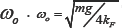 Then, the change in the vertical acceleration can be derived as [27-29]
Then, the change in the vertical acceleration can be derived as [27-29]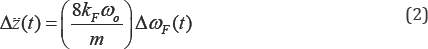
Thus, only the rotor's average angular speed, ωF(t), necessary to generate F (t) needs to be controlled to regulate the altitude, z(t) , of the quadrotor, since m ,and kF are g constants.
According to the AR. Drone 2.0 SDK documentation, z(t) is controlled by applying a reference vertical speed , as control input. The motion commands for the drone are encoded under
a specific protocol, where high-level control signals, including
, as control input. The motion commands for the drone are encoded under
a specific protocol, where high-level control signals, including 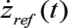 , are normalized between -1 and 1to prevent damage. The drone's flight management system sampling time, Ts , is 0.065 s, which is also the sampling time at which the control law is executed and the navigation data received.
, as control input. The motion commands for the drone are encoded under
a specific protocol, where high-level control signals, including , are normalized between -1 and 1to prevent damage. The drone's flight management system sampling time, Ts , is 0.065 s, which is also the sampling time at which the control law is executed and the navigation data received.
The control block diagram for the drone's altitude motion regulation is shown in Figure 3. The desired height and the actual system response are denoted zdes(t) and z(t) , respectively. The dynamics is implemented using (2), used to determine ωf(t) from the actual drone vertical speed, z(t) . The rotors rotate at equal speed,ωf(t) , which will generate F(t) to make z (t) reach the reference (zdes (t) = 1m). These computations take place in the on-board control system programmed in C. The simulation setup used is shown in Figure 4. The overall time delay,Td, single constant, in the system is represented as actuator time delay, as an explicit plant parameter. G(s) is the plant model for the combined motor and rigid body altitude dynamics without uncertainty effect.


Altitude Model and Design of Controllers
Altitude Model
Quadrotor altitude motion has second-order dynamics
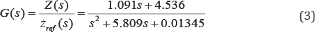
(Equation 1 & 2). Black-box approach was used to determine the model
for the drone altitude control. MATLAB system identification toolbox
App was applied to obtained LTI SISO ARX transfer function, stable
system, without time delay, as
Measured data, recorded from the drone's altitude
motion response, was imported into the App for the modeling process.The
input data was the reference vertical speed,
, constrained to [-1 1] m/s, and the output data was the vertical
height, z(t). A suitable P-feedback controller was used to obtain the
data. The model has a fit to estimation (best fit) of91.04%, final
prediction error (FPE) of 0.000200948, and mean squared error (MSE) of
0.0001864.The system is completely state controllable and completely
observable. See Figure 5 for the open-loop unit step response of the plant.
, constrained to [-1 1] m/s, and the output data was the vertical
height, z(t). A suitable P-feedback controller was used to obtain the
data. The model has a fit to estimation (best fit) of91.04%, final
prediction error (FPE) of 0.000200948, and mean squared error (MSE) of
0.0001864.The system is completely state controllable and completely
observable. See Figure 5 for the open-loop unit step response of the plant. 
Non-adaptive control: PV

The conceptual application of this control strategy
is common in angular position of DC motors, typically the control of
robot manipulators [30].
PV-control, unlike proportionalplus-derivative (PD) control, does not
induce numerator dynamics. The setup of the PV control system is shown
in Figure 6, where Kp and Kv
are the proportional (position) and velocity (derivative) gains,
respectively. The transfer function of the time-delay closed-loop system
is given as
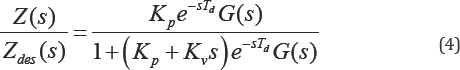
Note, if G(s)= 1/s, a first order plant, used in [19,20] for the estimation of the delay, then this time-delay system will be neutral type, see [21,22] for analysis of such control system. Also, if G(s)= 1/s and then we have a P-control,retarded type time-delay, system.
Adaptive control: PV-MRAC
The primary function of adaptive controller is to
accommodate uncertainties, which may introduce nonlinearities on the
system dynamics. There are several broad categories of AC, and in this
brief MRAC is applied. The type of MRAC depends on the adjustable
mechanism, and one of the modern ones is the MIT rule. The setup of the
MIT rule MRAC is shown in Figure 7, where Gp(s) and Gm(s) are transfer functions of the plant (including the uncertainties) and the reference model respectively, and yp(t) and ym(t) are their respectively outputs.

The reference signal is r(t) ,  is an updating parameter, γ> 0 is a tuning parameter, and the control input signal, u(t) — θ(t)r(t) , where n is the order of the system. The constant k
for the plant is unknown (e.g. is the effect of quadrotor payload
fluctuations or time-delay or both).CO is chosen as multiplied of Gm(s)by a desired constant, ka , so that and can matched. The tracking error, e(t)=yp(t)-ym(t),given by
is an updating parameter, γ> 0 is a tuning parameter, and the control input signal, u(t) — θ(t)r(t) , where n is the order of the system. The constant k
for the plant is unknown (e.g. is the effect of quadrotor payload
fluctuations or time-delay or both).CO is chosen as multiplied of Gm(s)by a desired constant, ka , so that and can matched. The tracking error, e(t)=yp(t)-ym(t),given by
Next is to define a cost function, J [θ(t)] , in
terms of e(t) . The goal here is to adjust θ(t) to minimize J related
to e(t) , so that as t increases e(t) → 0 . One simplest way is to
expressed [23,31-34]. The rule employs a feed-forward gain adaption to update θ , as shown below [23,32-34].
[23,31-34]. The rule employs a feed-forward gain adaption to update θ , as shown below [23,32-34].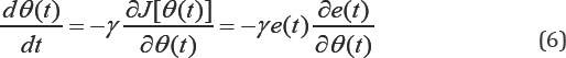
Where,  is sensitivity derivative of the system, and it is evaluated under assumption that θ varies slowly [23,33,34].
is sensitivity derivative of the system, and it is evaluated under assumption that θ varies slowly [23,33,34].
Now, θ(t)=[θ1(t)θ2(t)] since
quadrotor altitude motion dynamics is a second-order system, then . The
reference model is selected based on desired transient specifications,
given in the form as [23,32]
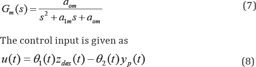
where r(t)=zdes(t). Substituting into (8), and simplifying, we obtain

And substituting (9) into (5), and then differentiating with respect θ1(t) and θ2(t) , to obtain
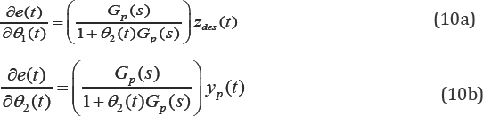
If the reference model is close to the plant, then their characteristic equations can be equally approximated  ,then the MIT update rule, from (6) and (10), can be written as
,then the MIT update rule, from (6) and (10), can be written as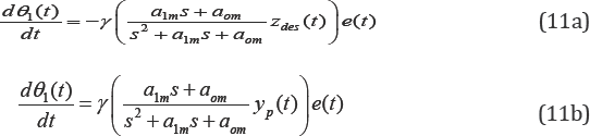
It is important to note that the MIT rule by itself does not guarantee error convergence or stability [23,32-34],
so the MRAC is combined with a tuned PV controller. An MRAC designed
using the MIT rule is very sensitive to the amplitudes of the signals.
As a general rule, the value of γ is kept small.Tuning of γ is crucial
to the adaptation rate and stability of the control system [23,32-34].
Simulations and Experiments
The MATLAB/Simulink program was developed for the experiments. The vertical speed control input constraints, [-1,1] ms(-1) , are applied using the saturation block. The estimated time delay of 0.36s obtained in [21,22]
was implemented using the transport delay block. The experiments were
conducted in an office environment with the drone's indoor hull
attached. The drone is connected to the host PC through WiFi (Figure 8).
Data streaming, commanding and reading, are done using UDPs. UDP is a
communication protocol that offers a limited amount of service when
messages are exchange between computers in a network that uses IP.

The drone navigation data (from the sensors, cameras,
battery, etc.) are received, and the control signals are sent, using AT
commands. AT commands are combination of short text strings sent to the
drone to control its actions. The drone has ultrasound sensor (at the
bottom) for ground altitude measurement. It has 1GHz 32-bit ARM Cortex
A8 processor, 1GB DDR2 RAM at 200MHz, and USB 2.0 high speed for
extensions. The drone�s total mass (including the indoor hull), m, is
453g.
Figure 9
shows the Simulink diagram developed for conducting the PV control
system simulations. For the PV control, a high pass filter (HPF) with
damping ratio,  was used for the derivative controller. A natural frequency value, ωf
=38 rad/s, for the filter was selected by tuning and the use of the
Bode plot. The filter�s cut off frequency was determined as 0.90 Hz. Figure 10
shows the Simulink diagram developed to simulate a unit-step response
for the PV-MRAC control system. The same HPF was applied in the control
system.
was used for the derivative controller. A natural frequency value, ωf
=38 rad/s, for the filter was selected by tuning and the use of the
Bode plot. The filter�s cut off frequency was determined as 0.90 Hz. Figure 10
shows the Simulink diagram developed to simulate a unit-step response
for the PV-MRAC control system. The same HPF was applied in the control
system.

Flight payload: disturbance rejection

To demonstrate the robustness of the PV-MRAC
controller, it was tested against the PV controller using the payload
capability of the drone. To accomplish this, the three cases below were
considered.
Case 1: point-mass load: before flight: Masking tape was used to attach point-mass loads at the top of the drone before (Figure 11).
The controllers were tested using different masses. This setup was used
to determine the stability bounds within which the changing
mass-inertia parameters of the system due to the acquired payload will
not destabilize the drone. The mass is assumed to be close to the
drone�s center of mass.
Case 2: cable-suspended point-mass load: Here,
a 100g point-mass load was attached to the end of an approximately 45cm
length of rope, which was hooked to the drone before flight (Figure 12).
Masking tape was used to hold firm the rope across the top and the
bottom of the drone. In this second case, apart from the drone carrying
an extra payload, the suspension system created an oscillating
(pendulum) disturbances to the system. The rope is assumed to be
massless and is attached to the drone�s center of mass.
apart from the drone carrying an extra payload, the
suspension system created an oscillating (pendulum) disturbances to the
system. The rope is assumed to be massless and is attached to the
drone's center of mass.

Case 3: point-mass load: during flight: In
this setup, the designed controllers were used to demonstrate the
stability behavior of the drone undergoing a range of instantaneous step
payload changes. Here, the masses were attached to a sticking masking
tape at the top of the drone, after it has stabilized to the desired
height, =1m, see Figure13.

Results and Discussion
The drone response contains a 'dead-time' due 1) time
delay in the control system and 2) the time between when the realtime
application from MATLAB/Simulink is connected to the drone and when the
controller is switched on. Consequently, for ease of analyzing the
experiments data, some of the drone's responses plots are shifted to
start at (0s,0m). For example, see Figure 14 for the drone altitude responses using a P-control system.

Note from Figure 14 that, for a P-control system, if there is no delay ( T d=0) in the system and KP > 0 , there should be no overshoot in the response. Also, increase in Kp should not destabilize the system. However, as seen in
Figure 14, when Kp >1, the output has a nonzero overshoot. Moreover, when Kp ≥ 5
, the amplitude of the response grows over time and the system becomes
unstable. This is partly due to the time delay in the system, which
introduces nonlinearity on the dynamics. Therefore, the delay does have
nontrivial effects on response and need be precisely estimated and
considered in designing effective control.
Non-adaptive control: pv
The controller gains were obtained by tuning. Figure 14 & 15 show the simulation and experimental responses, respectively. It can be observed that as the value kv value increases Mo decreases, but the responses becomes slower. The PV controller with kv= 0.3 and kp=2-0 gives the best stable control system performance, with rise time tr (10%-90%range) of 1.30 s and M0 = 2.03% .The results in Figure 16 and Table 1 compares simulated and experimented with and without the time-delay effects on the control system, with Kv = 03 and kv=2-0It
can be observed from the rise time values the importance of
incorporating the time delay into the design of the control system.


MATLAB-based software package [35] was used to study the equation, 1+(kp+KvS)e-stdG(s)
=0 , from (4). The closed-loop system stability of the time-delay
system, by solving the characteristic characteristic roots within a
specified region are then plotted for various kv values with k p= 2.0 . Figure 17
shows the shows the spectrum distribution of the characteristic roots.
When the rightmost (i.e., dominant) roots for each case are considered k
v- 0.3 the value yields the most stable rightmost root (
spectrum distribution of the characteristic roots. When the R(s)=-3.10).

Adaptive control: PV-MRAC
Figure 18&19 show simulated and experimented responses, respectively, for different values. It can be seen that, increasing γ makes the response faster but it introduces oscillations, while decreasing γ
makes the response slower leading to an unstable system. The results
show that there is a range of values of to achieve stabilization,
assuming the other tuning parameters remains constant. The results in Figure 20 and Table 2
compares simulated and experimented with and without the time-delay
effects. Here again, the results show the effect of including the time
delay in the control systems design. Note that, using the PV controller
and MRAC controller parameters on their own never stabilized the system.


Flight payload: disturbance rejection
Figure 21-23
show the responses for the three cases considered in introducing
disturbances to the drone, see Section 4.1. In general, the results
confirm that the PV-MRAC offers several benefits over the fixed-gain
approach, PV controller. The PV-MRAC was found to offer enhanced
robustness to the change in mass uncertainty and the oscillating
disturbances.


Case 1: point-mass load: before flight
Figure 21
shows the altitude responses for the PV and PV-MRAC controllers for the
case of attaching 130g point- mass load at the top of the drone. For
the PV-MRAC, it was observed that beyond 130g the oscillations were
larger, which destabilizes the drone. The drone's stability bounds
reached at 130g for the PV-MRAC. For the PV control, it can be seen that
with 130g attached, the drone was destabilized. The drone's stability
bounds reached at 120g for the PV control. The difference in performance
of the controllers was obvious, the adaptive controller allowed safe
operation and landing, while the PV controller failed to prevent
instability and sometimes resulted in a crash landing.
Case 2: cable-suspended point-mass load
The case of attaching 100g suspended point-mass load,
which introduced oscillating disturbances, both controllers achieved
the task of rising to the desired height, however, the PV-MRAC
controller still performed better, see Figure 22.
The PV-MRAC controller response has smaller oscillations about the
desired height value compared to the PV controller response.
Case 3: point-mass load: during flight
Figure 23
show the responses for the PV and PV-MRAC controllers, respectively,
for the case when instantaneous point-mass load of 135g was attached at
the top of the drone. As it can be observed, the PV controller failed to
prevent instability and resulted in a crash landing, but the adaptive
controller maintained the stability and allowed safe operation and
landing. The drone's stability bounds reached at 125g and 135g using the
PV and PV-MRAC controllers, respectively.
Conclusion
This paper has presented a second order LTI SISO ARX
altitude motion model, without time delay, for a quadrotor types of
UAVs. The effect of time delay on the drone's altitude response was
analysed including system stability conditions for the tuned PV control
system. The non-adaptive PV controller was designed for improved
transient responses based on the rightmost roots calculated using the
estimated delay value. Also, the MRAC based on the MIT rule was designed
by incorporating the time delay. The MRAC is combined with a tuned PV
controller, since the MIT rule MRAC on its own cannot guarantee
stability.?
The robustness of the PV-MRAC controller was
validated by comparing its performance to that of the non-adaptive PV
controller, using the payload capability of the drone and the
introduction of oscillating disturbances to the system. It was shown
that the PV-MRAC offers several benefits over the fixed- gain approach
of the PV controller. The PV-MRAC was found to offer enhanced robustness
to the parametric (uncertainty in mass) and the oscillating
disturbances. The difference in performance of the controllers was
obvious. The adaptive controller allowed safe operation and landing
while the PV controller failed to prevent instability and sometimes
resulted in a crash landing. The drone's stability bounds reached at
120g and 130g for added attached mass-inertia using the PV and PV-MRAC
controllers, respectively. In the case of the instantaneous introduction
of the mass-inertia, the drone's stability bounds reached at 125g and
135g using the PV and PV-MRAC controllers, respectively.
Future work could involve comparing the performance
of the MRAC based on the MIT rule to that based on the Lyapunov
stability arguments, including composite adaptation. Composite MRAC
adapts to both estimation and tracking errors. Also, multi-axis dynamics
of the drone system considering attitude and lateral motions (x and y)
can be considered. This problem is significantly more challenging, since
the equation of motions are coupled and more complex than that of the
altitude motion.
For More Open Access Journals Please Click on: Juniper Publishers
Fore More Articles Please Visit: Robotics & Automation Engineering Journal


Comments
Post a Comment