On the Alternatives of Lyapunov’s Direct Method in Adaptive Control Design- Juniper Publishers
Juniper Publishers- Journal of Robotics

Abstract
The prevailing methodology in designing adaptive
controllers for strongly nonlinear systems is based on Lyapunov’s PhD
Thesis he defended in 1892 to study the stability of motion of systems
for the solution of the equations of motion of which no closed form
analytical solutions exist. The adaptive robot controllers developed in
the nineties of the 20thcentury guarantee global (often asymptotic)
stability of the controlled system by using his ingenious Direct Method
that introduces a Lyapunov function for the behavior of which relatively
simple numerical limitations have to be proved. Though for various
problem classes typical Lyapunov function candidates are available, the
application of this method requires far more knowledge than the
implementation of some algorithm. Besides requiring creative designer’s
abilities, it often requires too much because it works with satisfactory
conditionsinstead of necessary and satisfactoryones. To evade these
difficulties, based on the firm mathematical background of constructing
convergent iterative sequences by contractive maps in Banach spaces, an
alternative of Lyapunov’s technique was so introduced for digital
controllers in 2008 that during one control cycle only one step of the
required iteration was done. Besides its simplicity the main advantage
of this approach was the possible evasion of complete state estimation
that normally is required in the Lyapunov function-based design. Though
the convergence of the control sequence can be guaranteed only within a
bounded basin, this approach seems to have considerable advantages. In
the paper the current state of the art of this approach is briefly
summarized.
Keywords: Adaptive control; Lyapunov function; Banach space; Fixed point lteration
Abbrevations: AC:
Adaptive Control; AFC: Acceleration Feedback Controller; AID: Adaptive
Inverse Dynamics Controller; CTC: Computed Torque Control; FPI: Fixed
Point Iteration; MRAC: Model Reference Adaptive Control; OC: Optimal
Control; PID:Proportional, Integrated, Derivative; RARC: Resolved
Acceleration Rate Control; RHC: Receding Horizon Controller;SLAC:
Slotine-Li Adaptive Controller;
Introduction
There is a wide class of model-based control
approaches in which the available approximate dynamic model of the
system to be controlled is “directly used” without “being inserted” into
the mathematical framework of “Optimal Control” (OC). A classical
example is the “Computed Torque Control” (CTC) for robots [1]. However,
in the practice we have to cope with the problem of the imprecision
(very often incompleteness) of the available system models (in robotics
e.g. [1,2], modeling friction phenomena e.g. [3-7], in life sciences as
modeling the glucose-insulin dynamics e.g. [8-11] or in anesthesia
control e.g. [12-14]). Modeling such engines as aircraft turbojet motors
is a quite complicated task that may need multiple model approach
[15-18]. Further practical problem is the existence and the consequences
of unknown and unpredictable “external disturbances”. A possible way of
coping with these practical difficulties is designing “Adaptive
Controllers” (AC) that somehow are able to observe and correct at least
the effects of the modeling imprecisions by “learning”. Depending on the
above available information on the model various adaptive methods can
be elaborated. If we have precise information on the kinematics of a
robot and only approximate information is available on the mass
distribution of a robot arm made of rigid links the exact model
parameters can be learned as in the case of the “Adaptive Inverse
Dynamics” (AID) and the “Slotine-Li Adaptive Controller” (SLAC) for
robots that are the direct adaptive extensions of the CTC control. An
alternative approach is the adaptive modification of the feedback gains
or terms [19]. The “Model Reference Adaptive Control” (MRAC) has double
“intent”: a) it has to provide precise trajectory tracking, and b) for
an outer, kinematics-based control loop they have to provide an illusion
that instead of the actually controlled system, a so called “reference
system” is under control (e.g. [20-22]).
The traditional approaches in controller design for
strongly nonlinear systems are based on the PhD thesis by Lyapunov [23]
that later was translated to Western languages (e.g. [24]). (In this
context “strong nonlinearity” means that the use of a “linearized system
model” in the vicinity of some “working point” is not satisfactory for
practical use.) In Lyapunov’s “2nd” or “Direct
Method” a Lyapunov function has to be constructed for the given
particular problem (typical “candidates” are available for typical
“problem classes”), and non-positiveness of the time-derivative of
this function has to be proved. Besides the fact that the creation
of the Lyapunov function is not a simple application of some
algorithm –it is rather some creative art–, this method has various
drawbacks as a) it works with “satisfactory conditions” instead
of “necessary and satisfactory conditions” (i.e. often it requires
too much as guaranteeing really not necessary conditions), b) its
main emphasis is on global (asymptotic) stability of the motion of
the controlled system without paying too much attention to the
“initial” or “transient” phase of the controlled motion (for instance
in life sciences a “transient” fluctuation can be lethal).
To cope with these difficulties alternatives of the Lyapunov
function-based adaptive design were suggested in [25] in
which the primary design intent is keeping at bay the initial
“transients” by turning the task of finding the necessary control
signal to iteratively so solving a fixed point problem [“Fixed Point
Iteration” (FPI)] that in each digital control step only one step
of the appropriate iteration can be realized. The mathematical
antecedents of this approach were established in the 17th century
(e.g. [26-28]), and its foundations in 1922 were extended to quite
complicated spaces by Stefan Banach [29,30]. In [25] the novelty
was the application of this approach to control problems. In
contrast to the “traditional” “Resolved Acceleration Rate Control”
(RARC) in which in the control of a 2nd order physical system only
lower order derivatives or tracking error integrals are fed back
(e.g. [19,31-33]) in this approach the measured “acceleration”
signals are also used as in the “Acceleration Feedback Controllers”
(AFC) (e.g. [34-38]).
In general, the most important “weak point” of the FPI-based
approach is that it cannot guarantee global stability. The generated
iterative control sequences converge to the solution of the control
task only within a bounded basin that in principle can be left. To
avoid this problem heuristic tuning rules were introduced for one
of the little numbers of the adaptive parameters in [39-41]. In
[42] essentially the same method was introduced in the design of
a novel type of MRAC controllers the applicability of which was
investigated by simulations for the control of various systems
(e.g. [43-46]). Observing the fact that in the classical, Lyapunov
function-based solutions as the AID and SLAC controllers the
parameter tuning rule obtained from the Lyapunov function has
a simple geometric interpretation that is independent of the
Lyapunov function itself, the FPI-based solution was combined
with the tuning rule of the original solutions used for learning the
“exact dynamic parameters” of the controlled system. Alleviated
from the burden of necessarily constructing some easily treatable
quadratic Lyapunov function, the feedback provided by the FPIbased
solution was directly used for parameter tuning. This
solution resulted in precise trajectory tracking even in the initial
phase of the learning process in which the available approximate
model parameters still were very imprecise [47,48]. In the present
paper certain novel results are summarized on the further
development of the FPI-based approach.
Discussion and Results
The structure of the FPI-based adaptive control
The block scheme of the FPI-based adaptive controller is given
in Figure 1 for a 2nd order dynamical system as e.g. a robot [48].
In this case the 2nd time-derivative of the generalized coordinates
(joint coordinates). qcan be instantaneously set by the control
torque or force Q On this basis, in the kinematic block an
arbitrary desired joint acceleration  can be designed that can
drive the tracking error N q (t) − q(t) to 0 if it is realized. In the practice
this joint acceleration cannot be realized due to the imprecisions
in the dynamic model the CTC controller uses for the calculation
of the necessary forces. Therefore, instead introducing this signal
into the Approximate Model to calculate the necessary force
its deformed version,
can be designed that can
drive the tracking error N q (t) − q(t) to 0 if it is realized. In the practice
this joint acceleration cannot be realized due to the imprecisions
in the dynamic model the CTC controller uses for the calculation
of the necessary forces. Therefore, instead introducing this signal
into the Approximate Model to calculate the necessary force
its deformed version,  is introduced into it. The necessary
deformation iteratively is produced in the form of a sequence that
is initiated by it, i.e. by During one digital control step one step
of the iteration can be realized. If there are no special time-delay
effects in the system, the contents of the delay boxes in Figure
1 exactly correspond to the cycle time of the controller Δt The
“chain of operations” resulting in an observed realized response
q(t) for the input mathematically approximately can be
considered as a response
is introduced into it. The necessary
deformation iteratively is produced in the form of a sequence that
is initiated by it, i.e. by During one digital control step one step
of the iteration can be realized. If there are no special time-delay
effects in the system, the contents of the delay boxes in Figure
1 exactly correspond to the cycle time of the controller Δt The
“chain of operations” resulting in an observed realized response
q(t) for the input mathematically approximately can be
considered as a response  since –though it depends on
q and q − only slowly varies in comparison to that quite
quickly can be modified. In the Adaptive Deformation Block of
Figure 1 a function is used as
since –though it depends on
q and q − only slowly varies in comparison to that quite
quickly can be modified. In the Adaptive Deformation Block of
Figure 1 a function is used as 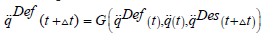 in
which
in
which 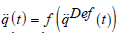 [49]. Since due to the proportional, integral
and derivative error feedback terms varies only slowly, we
have an approximation as
[49]. Since due to the proportional, integral
and derivative error feedback terms varies only slowly, we
have an approximation as 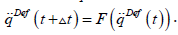 Regarding the
convergence of this iteration, we have to take it into account
that a Banach Space (accidentally denoted by B is a complete,
linear, normed metric space. It is a convenient modeling tool
that allows the use of simple norm estimations. Its completeness
means that each self-convergent or Cauchy sequence has a limit
point within the space. A mapping F :β β is contractive if ∃
a real number 0 ≤ K < 1 so that,
Regarding the
convergence of this iteration, we have to take it into account
that a Banach Space (accidentally denoted by B is a complete,
linear, normed metric space. It is a convenient modeling tool
that allows the use of simple norm estimations. Its completeness
means that each self-convergent or Cauchy sequence has a limit
point within the space. A mapping F :β β is contractive if ∃
a real number 0 ≤ K < 1 so that,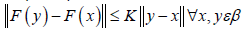 It is easy to show that the sequence generated by a contractive
map as
It is easy to show that the sequence generated by a contractive
map as 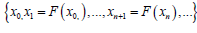 is a Cauchy sequence: in the norm
estimation given in (1)∀Lε in high order powers of K occur as
n → ∞ therefore
is a Cauchy sequence: in the norm
estimation given in (1)∀Lε in high order powers of K occur as
n → ∞ therefore 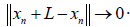 Due to the completeness of
  arbitrary element of the sequence n x according to (2) it holds that
 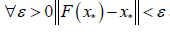 .
.
can be designed that can
drive the tracking error N q (t) − q(t) to 0 if it is realized. In the practice
this joint acceleration cannot be realized due to the imprecisions
in the dynamic model the CTC controller uses for the calculation
of the necessary forces. Therefore, instead introducing this signal
into the Approximate Model to calculate the necessary force
its deformed version, is introduced into it. The necessary
deformation iteratively is produced in the form of a sequence that
is initiated by it, i.e. by During one digital control step one step
of the iteration can be realized. If there are no special time-delay
effects in the system, the contents of the delay boxes in Figure
1 exactly correspond to the cycle time of the controller Δt The
“chain of operations” resulting in an observed realized response
q(t) for the input mathematically approximately can be
considered as a response since –though it depends on
q and q − only slowly varies in comparison to that quite
quickly can be modified. In the Adaptive Deformation Block of
Figure 1 a function is used as in
which [49]. Since due to the proportional, integral
and derivative error feedback terms varies only slowly, we
have an approximation as Regarding the
convergence of this iteration, we have to take it into account
that a Banach Space (accidentally denoted by B is a complete,
linear, normed metric space. It is a convenient modeling tool
that allows the use of simple norm estimations. Its completeness
means that each self-convergent or Cauchy sequence has a limit
point within the space. A mapping F :β β is contractive if ∃
a real number 0 ≤ K < 1 so that, It is easy to show that the sequence generated by a contractive
map as is a Cauchy sequence: in the norm
estimation given in (1)∀Lε in high order powers of K occur as
n → ∞ therefore Due to the completeness of arbitrary element of the sequence n x according to (2) it holds that .


Consequently, it is enough to guarantee that the function F(.) is
contractive, since in this case the sequence converges to the fixed
point of this function if it is so constructed that its fixed point is the
solution of the control task.
Construction of the adaptive function
In the original solution in [25] (3) was suggested for the
special case qε IRwith three adaptive parameters Kc, Bc, and Ac.

Really, when 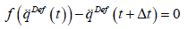 we just have
the solution of the control task and it is obtained that
we just have
the solution of the control task and it is obtained that 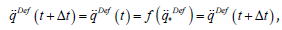 that is the solution is a fixed
point. To obtain convergence in the vicinity of the fixed consider
the 1st order Taylor series approximation as
that is the solution is a fixed
point. To obtain convergence in the vicinity of the fixed consider
the 1st order Taylor series approximation as
we just have
the solution of the control task and it is obtained that that is the solution is a fixed
point. To obtain convergence in the vicinity of the fixed consider
the 1st order Taylor series approximation as
leads to the approximation

On the basis of (5) it is easy to set the adaptive parameters for
convergence: by choosing a great parameter 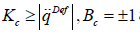 and a small Ac it can be achieved that
 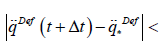 therefore
the mapping is contractive and the sequence converges to the
solution. The speed of convergence depends on setting Ac, and too
great value can cause leaving the region of convergence.
therefore
the mapping is contractive and the sequence converges to the
solution. The speed of convergence depends on setting Ac, and too
great value can cause leaving the region of convergence.
and a small Ac it can be achieved that therefore
the mapping is contractive and the sequence converges to the
solution. The speed of convergence depends on setting Ac, and too
great value can cause leaving the region of convergence.
For qε IRn (multiple variable systems) a different construction
was introduced in [50,51] the convergence properties of which
were more lucid than that of the multiple variable variant of (3):

in which the expression 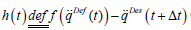 can be
identified as the “response error in time t”, and with the Frobenius
norm
can be
identified as the “response error in time t”, and with the Frobenius
norm  corresponds to the unit vector that is directed into
the direction of the response error, ζ : IR IR is a differentiable
contractive map with the attractive fixed point ( )* * ζ x = x and
c Aε IR is an adaptive control parameter. By using the same
argumentation with the1st order Taylor series approximation it
was shown in [52] that if the real part of each eigenvalue of
corresponds to the unit vector that is directed into
the direction of the response error, ζ : IR IR is a differentiable
contractive map with the attractive fixed point ( )* * ζ x = x and
c Aε IR is an adaptive control parameter. By using the same
argumentation with the1st order Taylor series approximation it
was shown in [52] that if the real part of each eigenvalue of  is
simultaneously positive or negative, an appropriate Ac parameter
can be selected that guarantees convergence.
is
simultaneously positive or negative, an appropriate Ac parameter
can be selected that guarantees convergence.
can be
identified as the “response error in time t”, and with the Frobenius
norm corresponds to the unit vector that is directed into
the direction of the response error, ζ : IR IR is a differentiable
contractive map with the attractive fixed point ( )* * ζ x = x and
c Aε IR is an adaptive control parameter. By using the same
argumentation with the1st order Taylor series approximation it
was shown in [52] that if the real part of each eigenvalue of is
simultaneously positive or negative, an appropriate Ac parameter
can be selected that guarantees convergence. 
in which Qε IR2 denotes the control force and qε IR2 is the array
of the generalized coordinates of the controlled system.
The parameter 1 σ , and
2 σ > 0 “modulate” the springs’
stiffness, the direction of the spring force is calculated by the use
of the “signum” function as sign ( ) 1 01 q − L while its absolute value is  The approximate and exact model parameter values are
given in Table 1.
The approximate and exact model parameter values are
given in Table 1.
The approximate and exact model parameter values are
given in Table 1.
In the Kinematic Block for the integrated error 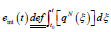 the prescribed “tracking strategy” was
  that lead to a PID-type
feedback
that lead to a PID-type
feedback  that choice guarantees
the convergence
that choice guarantees
the convergence  in the simulations ∧ = 6s−1
was chosen with ζ (x) = atanh (tanh (x + D) / 2),D = 0.3 in (6). The choice
5 10 1 c A = − × − resulted in good convergence. The Figure2–6 illustrate
the effects of using the adaptive deformation. It is evident that
the tracking precision was considerably improved without any
chattering effect that are typical in the also simple Sliding Mode
/ Variable Structure Controllers (e.g. [53,54]. Figure 5 reveals that
quite different control forces were applied in the non-adaptive
and in the adaptive cases.
in the simulations ∧ = 6s−1
was chosen with ζ (x) = atanh (tanh (x + D) / 2),D = 0.3 in (6). The choice
5 10 1 c A = − × − resulted in good convergence. The Figure2–6 illustrate
the effects of using the adaptive deformation. It is evident that
the tracking precision was considerably improved without any
chattering effect that are typical in the also simple Sliding Mode
/ Variable Structure Controllers (e.g. [53,54]. Figure 5 reveals that
quite different control forces were applied in the non-adaptive
and in the adaptive cases.
the prescribed “tracking strategy” was that lead to a PID-type
feedback that choice guarantees
the convergence in the simulations ∧ = 6s−1
was chosen with ζ (x) = atanh (tanh (x + D) / 2),D = 0.3 in (6). The choice
5 10 1 c A = − × − resulted in good convergence. The Figure2–6 illustrate
the effects of using the adaptive deformation. It is evident that
the tracking precision was considerably improved without any
chattering effect that are typical in the also simple Sliding Mode
/ Variable Structure Controllers (e.g. [53,54]. Figure 5 reveals that
quite different control forces were applied in the non-adaptive
and in the adaptive cases.


The essence of the adaptivity is revealed by Figure 6. In the
non-adaptive case considerable PID corrections are added to therefore it considerably differs fromthat is identical to in the lack of adaptive deformation. However, the difference
between the desired and the realized 2nd time-derivatives are quite
considerable if no adaptive deformation is applied. In contrast to
that, in the adaptive caseis in the vicinity of because
only small PID corrections are needed if the trajectory tracking is
precise. This desired value is very close to the realized 2nd time
derivatives that considerably differ from the adaptively deformed
value. That is, quite considerable adaptive deformation was
needed for precise trajectory tracking due to the great modeling
errors.
therefore it considerably differs fromthat is identical to in the lack of adaptive deformation. However, the difference
between the desired and the realized 2nd time-derivatives are quite
considerable if no adaptive deformation is applied. In contrast to
that, in the adaptive caseis in the vicinity of because
only small PID corrections are needed if the trajectory tracking is
precise. This desired value is very close to the realized 2nd time
derivatives that considerably differ from the adaptively deformed
value. That is, quite considerable adaptive deformation was
needed for precise trajectory tracking due to the great modeling
errors. Further Possible Applications and Development
The applicability of the FPI-based adaptive control design
methodology was investigated in various potential fields of
application. In 2012 in [55] an adaptive emission control of freeway traffic was suggested by the use of the quasistationary
solutions of an approximate hydrodynamic traffic model. In [56]
an FPI-based adaptive control problem of relative order 4 was
investigated. In [57] FPI-based control of the Hodgkin-Huxley
Neuron was considered. In [58] the possible regulation of Propofol
administration through wavelet-based FPI control in anaesthesia
control was investigated.
In [59] the application of the FPI-based control in treating
patients suffering from “Type 1 Diabetes Mellitus” was studied.
The simplicity of the FPI-based method opened new prospects
in the possible design of adaptive optimal controllers. In [60]
the contradiction between the various requirements in OC was
resolved in the case of underactuated mechanical systems in
the following manner: instead constructing a “cost function
contribution” to each state variable the motion of which needed
control, consecutive time slots were introduced within which
only one of the state variables was controlled with FPI-based
adaptation. (The different sections may correspond to different
relative order control tasks.) In [61] it was pointed out that the
FPI-based control can be easily combined with the mathematical
framework of the “Receding Horizon Controllers” (RHC) (e.g.
[62]). (A combination with the Lyapunov function-based adaptive
approach would be far less plausible and simple.) In [49] the
applicability of this approach was introduced into the control
of systems with time-delay. The possibility of fractional order
kinematic trajectory tracking prescription in the FPI-based
adaptive control was studied, too [63].
In [64] its applicability was investigated in treating angiogenic
tumors. In [65,66] further simplification of the adaptive RHC
control was considered in which the reduced gradient algorithm
was replace by a FPI
in finding the zero gradient of the “Auxiliary Function” of the
problem. In [67] the applicability of the method was experimentally
verified in the adaptive control of a pulse-width modulation driven
brushless DC motor that did not have satisfactory documentation
(FIT0441 Brushless DC Motor with Encoder and Driver) and
was braked by external forces simply by periodically grabbing
the rotating shaft by one’s two fingers. The solution was based
on a simple Arduino UNO microcontroller with embedding the
adaptive function defined in (3) into the motor’s control algorithm.
In spite of using 2nd time-derivatives in the feedback no special
noise filtering was applied. The measured and computed data was
visualized by a common laptop. As it can be seen in Figure 7, the
rotational speed was kept at almost constant (in spite of the very
noisy measurement data), and the adaptive deformation and the
control signal were well adapted to the external braking forces in
harmony with the simulation results belonging to the “Illustrative
Example” in subsection 2.3.

Figure 7: The experimental setup used for the verification
of the FPI-based adaptive control in the case of a pulse-width
modulated brushless electric DC motor; The nominal and the
realized rotational speed (the average of the whole data set
was 59:9383rpm, the nominal constant value was 60rpm); The
“Desired” and adaptively “Deformed” 2nd timederivatives of the
rotational speed; The control signal (from [67], courtesy of Tamás
Faitli) In [68] the novel adaptive control approach was considered
from the side of the Lyapunov function-based technique and it
was found that it can be interpreted as a novel methodology that
is able to drive the Lyapunov function near zero and keeping it
in its vicinity afterwards. On this basis a new MRAC controller
design was suggested in [69] that has similarity with the idea of
the “Backstepping Controller” [70,71].
Conclusion
The FPI-based adaptive control approach was introduced at
the Óbuda University with the aim of evading the mathematical
difficulties and restrictions, furthermore the information need
related to the traditional Lyapunov function-based design. Its main point was the transformation of the control task into a
fixed-point problem that was iteratively solved on the firm
mathematical basis of Banach’s fixed point theorem. In the center
of the new approach, instead of the requirement of global stability,
as the primary design intent, precise realization of a kinematically
(kinetically) prescribed tracking error relaxation was placed. In
contrast to the traditional soft computing approaches as fuzzy,
neural network and neuro-fuzzy solutions that normally apply
huge structures with ample number of the parameters of the
universal approximators of the continuous multiple variable
functions on the basis of Kolmogorov’s approximation theorem
(e.g.
[72-74]) this approach has only a few independent adaptive
parameters that can be easily set and one of them can be tuned
for maintaining the convergence of the control algorithm. It was
shown that the simplicity of this approach allows its combination
with more “traditional” approaches as that learning the exact
model parameters of the controlled system and at various levels
of the optimal controllers as the RFC control. On the basis of ample
simulation investigations, it can be stated that the suggested
approach has wide area of potential applications (in the control
of mechanical devices, in life sciences, traffic control, etc.) where
the presence of essential nonlinearities, the lack of precise and
complete system models, and limited possibilities for obtaining
information on the controlled system’s state are present as main
difficulties. It seems to be expedient to invest more efforts into
experimental investigations.
Acknowledgement
The Authors express their gratitudes to the Antal Bejczy
Center for Intelligent Robotics, and the Doctoral School of Applied
Informatics and Applied Mathematics for supporting their work.
For More Open Access Journals Please Click on: Juniper Publishers
Fore More Articles Please Visit: Robotics & Automation Engineering Journal


Comments
Post a Comment